Preparation

You can request your entire spotify playback history data from spotify from this link https://spotify.com/us/account/privacy/. Note that you can get your playback history for the past year within 5 days. Once you make the request, for safety reason Spotify will be sending you an email to verify that it was you who requested this copy of the data. It is necessary to confirm the email you receive. After that, you just need to follow the instructions and download the data.

You will find a folder called “My Data” which contains different files in JSON format, including a very particular one which is your playback history, with the file name “StreamingHistory0.json”. In case of having more intense playback hour, you will more likely to have “StreamingHistory1.json”, “StreamingHistory2.json” and so on. In my case, I have 3 of them.

I hate wroking with json but jsonlite make things easier to work with json in R. I use several R packages, but the most essential packages are tidyverse and jsonlite. Alright, we are now ready and let’s move to R.

Setup in R

library(here) #It's here, hehehe
library(jsonlite) #I hate working with JSON in R, but this package make things easier
library(lubridate) 
library(gghighlight)
library(tidyverse) #O'holy tidiverse
library(knitr)
library(plotly) #You are going to love this package, try it!
library(ggrepel)
library(MetBrewer)
library(RColorBrewer)
library(wesanderson)
library(viridis)

here() # checking the directory
streamhistory <- fromJSON("/Users/edodanilyan/Documents/analisis data client/MyData/StreamingHistory0.json", flatten = TRUE)
streamhistory1 <- fromJSON("/Users/edodanilyan/Documents/analisis data client/MyData/StreamingHistory1.json", flatten = TRUE)
streamhistory2 <- fromJSON("/Users/edodanilyan/Documents/analisis data client/MyData/StreamingHistory2.json", flatten = TRUE)

head(streamhistory)

Adding time to the dataset

myspotify <- streamhistory %>% 
  as_tibble() %>% 
  mutate_at("endTime", ymd_hm) %>% 
  mutate(endTime = endTime - hours(6)) %>% 
  mutate(date = floor_date(endTime, "day") %>% as_date, seconds = msPlayed / 1000, minutes = seconds / 60)
myspotify1 <- streamhistory1 %>% 
  as_tibble() %>% 
  mutate_at("endTime", ymd_hm) %>% 
  mutate(endTime = endTime - hours(6)) %>% 
  mutate(date = floor_date(endTime, "day") %>% as_date, seconds = msPlayed / 1000, minutes = seconds / 60)
myspotify2 <- streamhistory2 %>% 
  as_tibble() %>% 
  mutate_at("endTime", ymd_hm) %>% 
  mutate(endTime = endTime - hours(6)) %>% 
  mutate(date = floor_date(endTime, "day") %>% as_date, seconds = msPlayed / 1000, minutes = seconds / 60)

myspotify <- rbind(myspotify, myspotify1, myspotify2) 

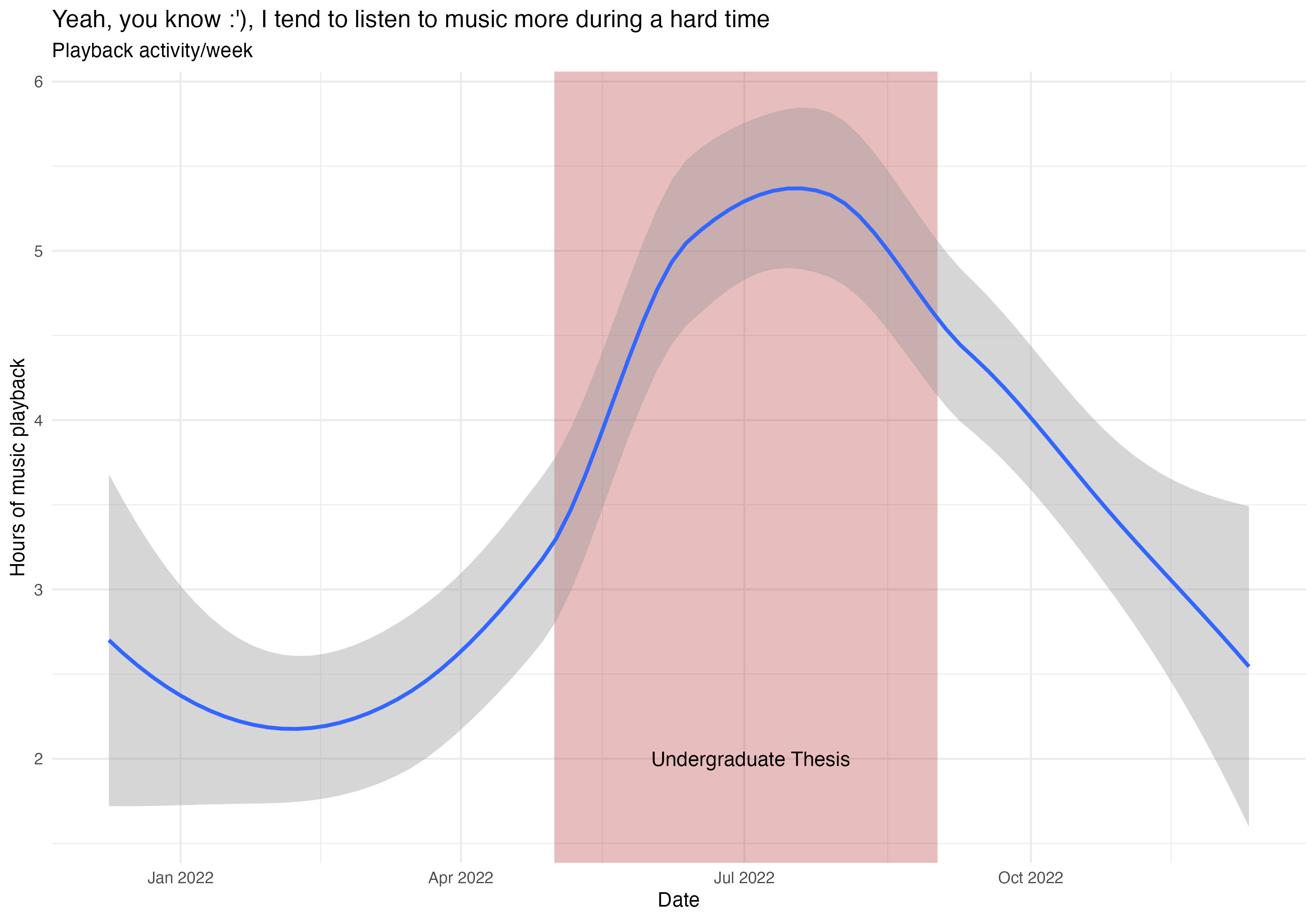
Playback activity per week

streaminghours <- myspotify %>% 
  filter(date >= "2020-01-01") %>% 
  group_by(date) %>% 
  group_by(date = floor_date(date, "week")) %>%
  summarize(hours = sum(minutes) / 60) %>% 
  arrange(date) %>% 
  ggplot(aes(x = date, y = hours)) + 
  geom_smooth(method = "loess") +
  scale_fill_manual() + 
  labs(x= "Date", y= "Hours of music playback") + 
  ggtitle("On what dates I've listened to more or less music on Spotify?", "Playback activity per week")+
  theme_minimal()

streaminghoursdata <- myspotify %>% 
  filter(date >= "2020-01-01") %>% 
  group_by(date) %>% 
  summarize(hours = sum(minutes) / 60) %>% 
  arrange(date)

xmin <- as.Date("2022-05-01")
xmax <- as.Date("2022-09-01")
xthesis <- as.Date("2022-06-01")

streaminghours <- ggplot(streaminghoursdata, aes(x = date, y = hours)) + 
  annotate("rect", fill = "firebrick", alpha = 0.3, 
           xmin = xmin, xmax = xmax,
           ymin = -Inf, ymax = Inf) +
  geom_smooth(method = "loess") +
  scale_fill_manual() + 
  annotate(geom = "text", x = xthesis, y = 2, label = "Undergraduate Thesis", hjust = "left")+
  labs(x= "Date", y= "Hours of music playback") + 
  ggtitle("Yeah, you know :'), I tend to listen to music more during a hard time", "Playback activity/week")+
  theme_minimal()
streaminghours

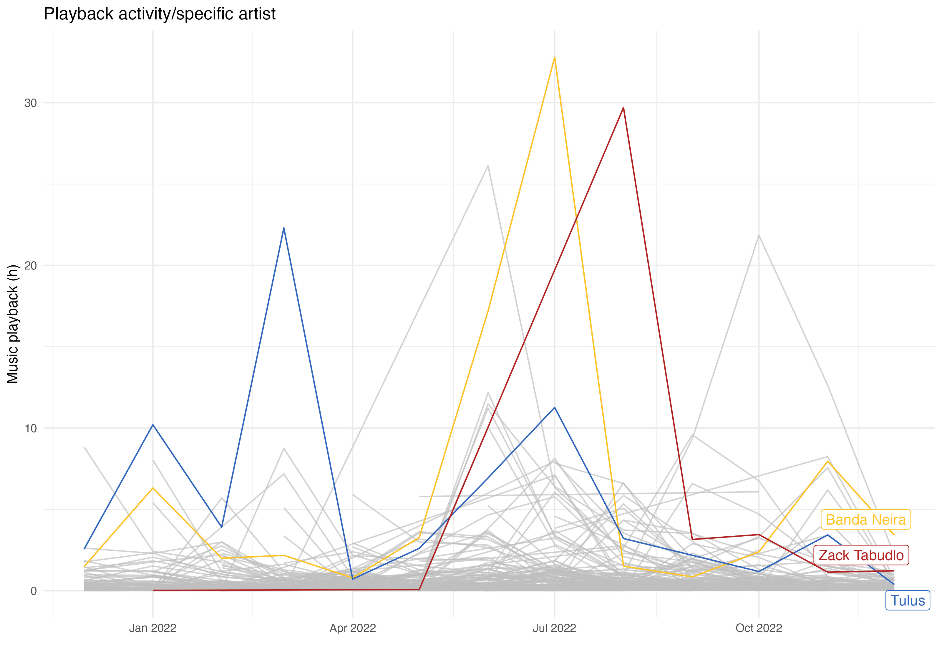
Playback activity per particular artist

hoursartist <- myspotify %>% 
  group_by(artistName, date = floor_date(date, "month")) %>% 
  summarize(hours = sum(minutes) / 60) %>% 
  ggplot(aes(x = date, y = hours, group = artistName, color = artistName)) + 
  labs(x= "Date", y= "Music playback (h)") + 
  ggtitle("Playback activity/specific artist") +
  geom_line(method = "loess", se = F) + 
  gghighlight(artistName == "Banda Neira" || artistName == "Tulus" || artistName == "Zack Tabudlo") +
  xlab("")+
  scale_color_manual(values = c("#ffc425", "#3066be", "firebrick")) +
  theme_minimal()
hoursartist

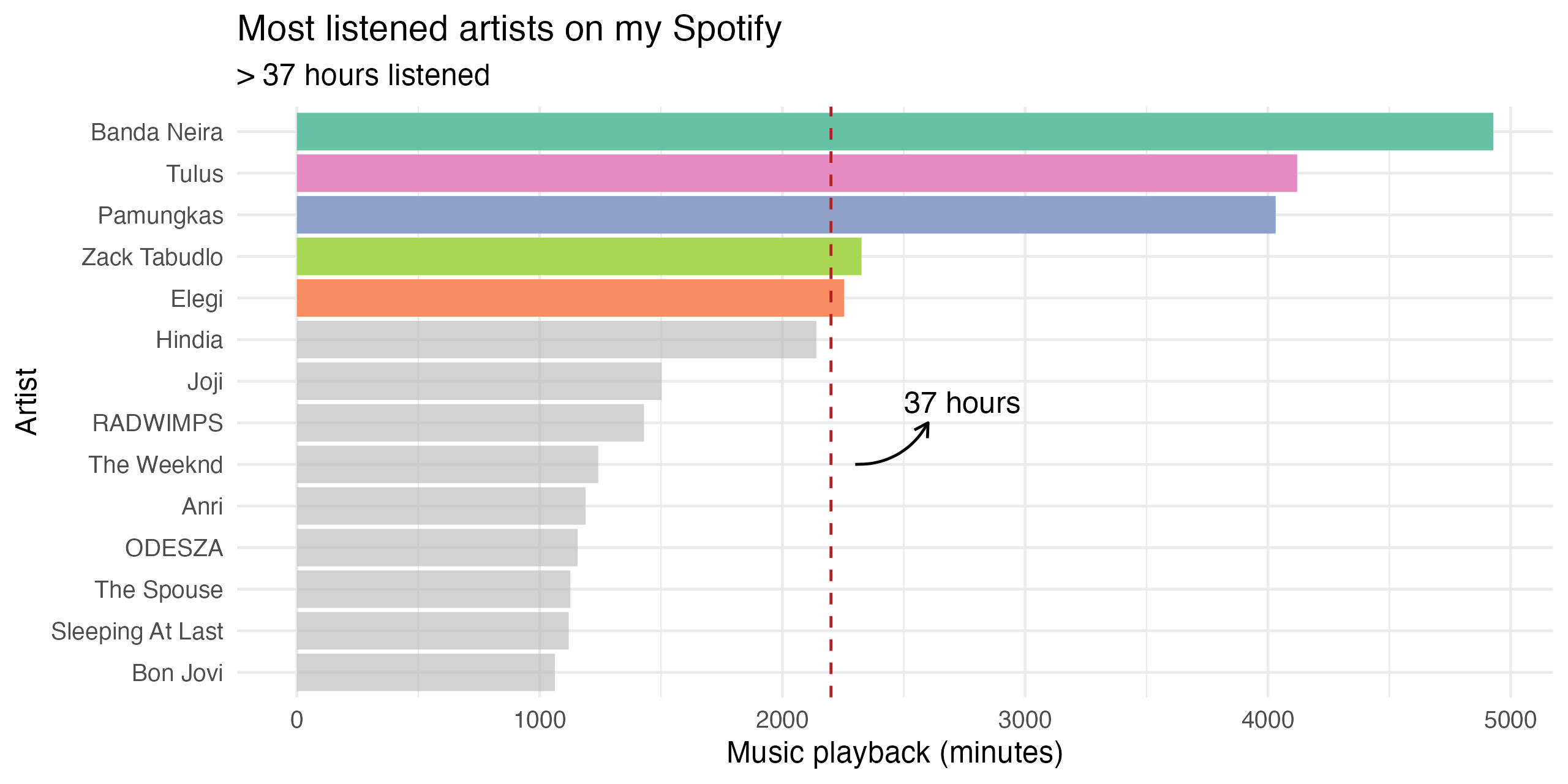
Most listened artist (more than 37 hours)

minutesmostlistened <- myspotify %>% 
  filter(date >= "2020-01-01") %>% 
  group_by(artistName) %>% 
  summarize(minutesListened = sum(minutes)) %>% 
  filter(minutesListened >= 1000) %>%
  ggplot(aes(reorder(x = artistName, minutesListened), y = minutesListened)) + 
  geom_col(aes(fill = artistName)) +
  scale_fill_brewer(palette = "Set2")+
  labs(x= "Artist", y= "Music playback (minutes)") + 
  ggtitle("Most listened artists on my Spotify", "> 37 hours listened") +
  theme(axis.text.x = element_text(angle = 90), legend.position = "none")+
  guides(fill = "none") +
  gghighlight(max(minutesListened) > 2200)+
  theme_minimal() +
  geom_hline(yintercept=2200, color="firebrick", linetype="dashed",
             size=.5)+
  annotate(
    geom = "curve", x = 6, y = 2300, xend = 7, yend = 2600, 
    curvature = .3, arrow = arrow(length = unit(2, "mm"))
  ) +
  annotate(geom = "text", x = 7.5, y = 2500, label = "37 hours", hjust = "left")+
  coord_flip()
minutesmostlistened

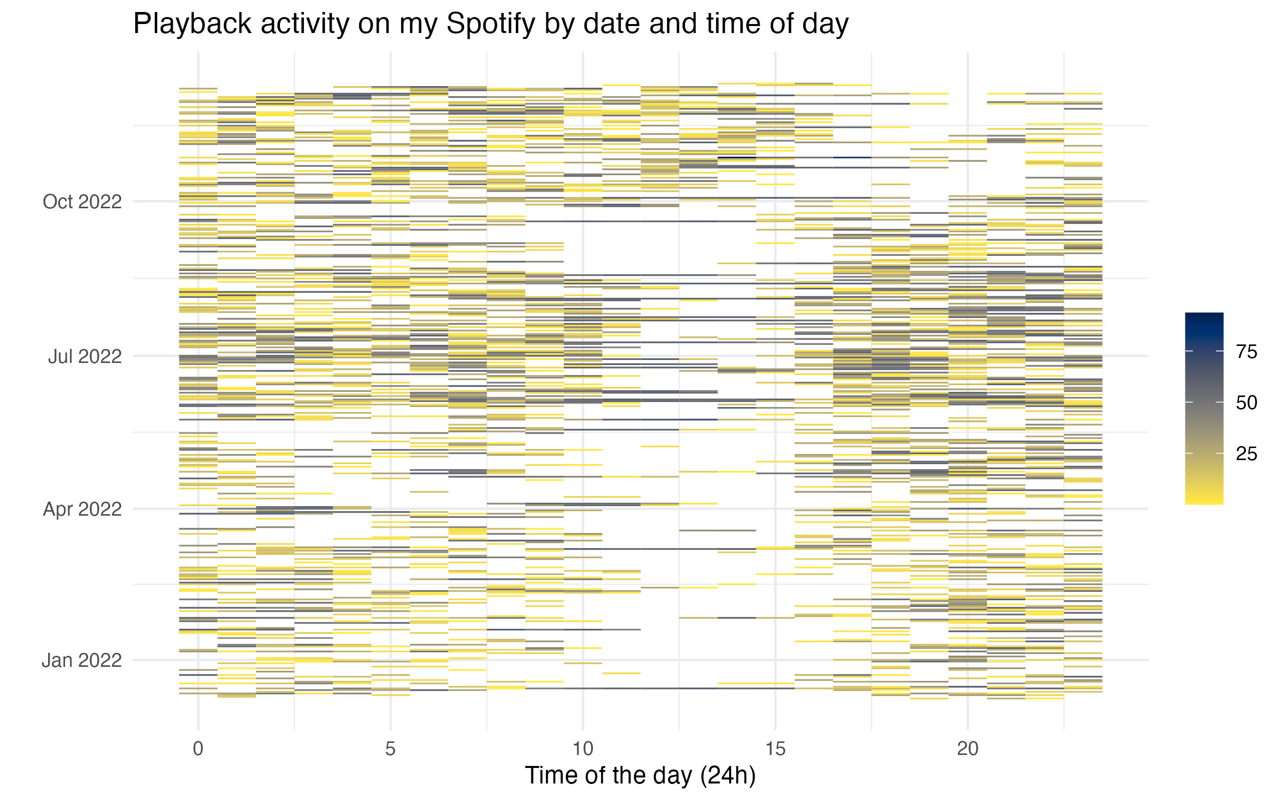
Playback activity by date and time of day

timeday <- myspotify %>% 
  filter(date >= "2020-01-01") %>% 
  group_by(date, hour = hour(endTime)) %>% 
  summarize(minutesListened = sum(minutes)) %>% 
  ggplot(aes(x = hour, y = date, fill = minutesListened)) + 
  geom_tile() + 
  labs(x= "Time of the day (24h)") + 
  ggtitle("Playback activity on my Spotify by date and time of day") +
  scale_fill_viridis(
    option = "cividis", direction = -1,
    name = "") +
  ylab("")+
  theme_minimal()
timeday

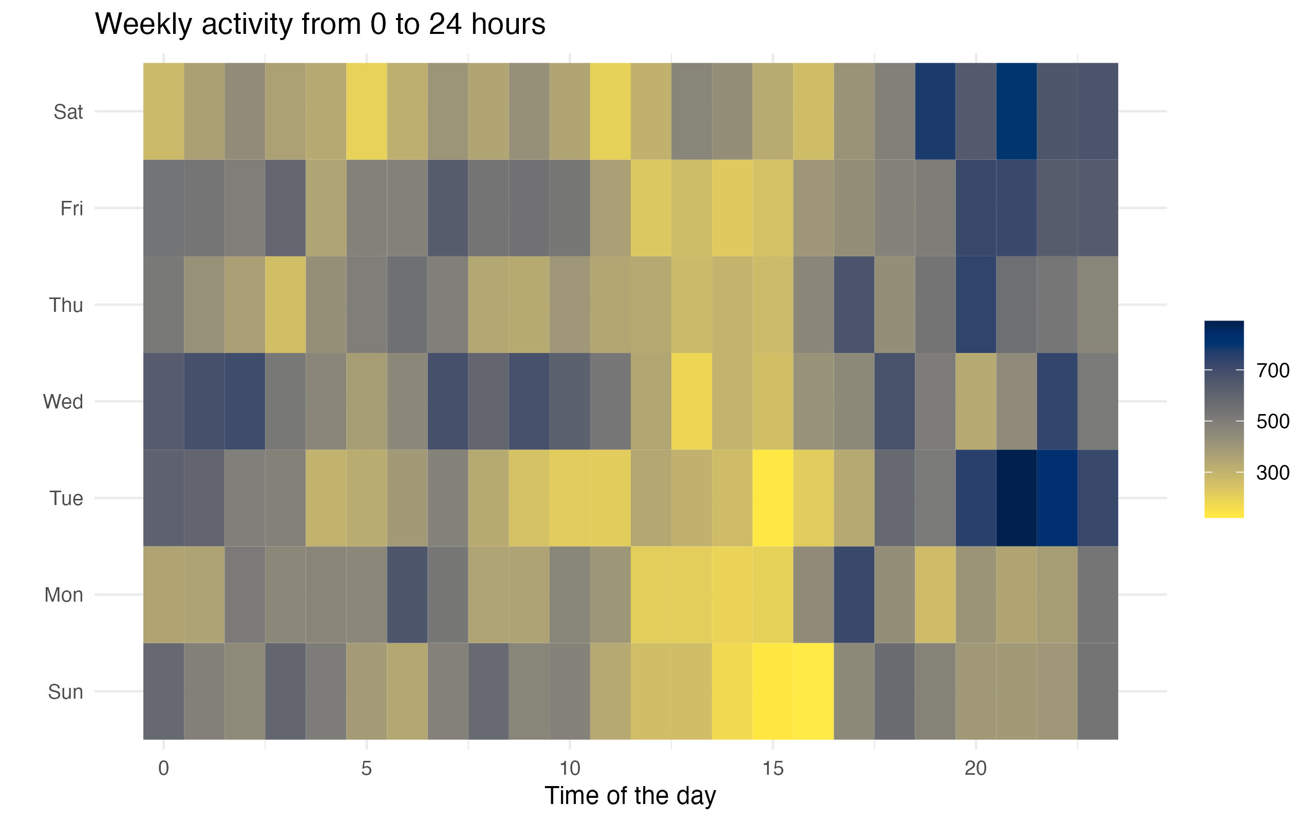
Weekly activity from 0 to 24 hours

hoursday <- myspotify %>% 
  filter(date > "2019-01-01") %>% 
  group_by(date, hour = hour(endTime), weekday = wday(date, label = TRUE))%>% 
  summarize(minutesListened = sum(minutes))

plothoursday <- hoursday %>% 
  group_by(weekday, hour) %>% 
  summarize(minutes = sum(minutesListened)) %>% 
  ggplot(aes(x = hour, weekday, fill = minutes)) + 
  geom_tile() + 
  scale_fill_viridis(
    option = "cividis", direction = -1,
    name = "") +
  labs(x= "Time of the day", y= "") + 
  ggtitle("Weekly activity from 0 to 24 hours")+
  theme_minimal()
plothoursday

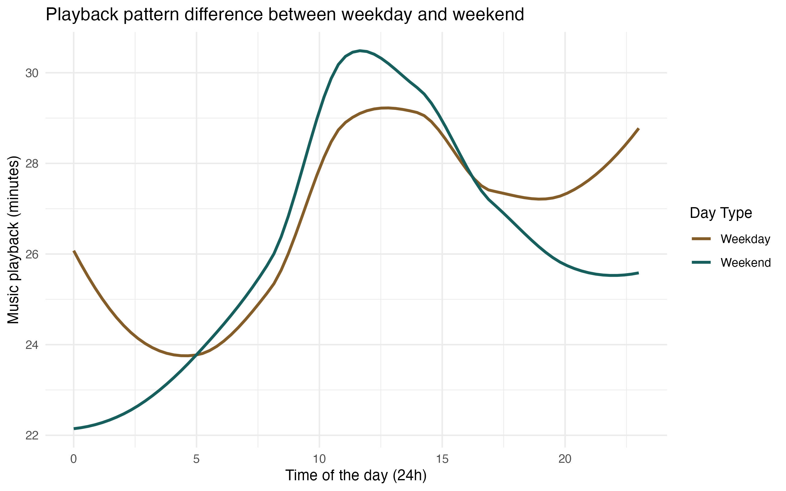
Playback pattern difference between weekday and weekend

hoursday <- hoursday %>% 
  mutate(day_type = if_else(weekday %in% c("Sat", "Sun"), "Weekend", "Weekday")) %>% 
  group_by(day_type, hour) %>% 
  summarize(minutes = mean(minutesListened))

daytype <- hoursday %>% 
  ggplot(aes(x = hour, y = minutes, color = day_type)) + 
  geom_smooth(method = "loess",size = 1, se = F) +
  scale_color_manual(values = c("#845d29",  "#175f5d"))+
  labs(x= "Time of the day (24h)", y= "Music playback (minutes)", color = "Day Type") + 
  ggtitle("Playback pattern difference between weekday and weekend") +
  theme_minimal()
daytype

Note: This is the most enjoyable personal project because I can see and understand the pattern of my spotify playback :D.

Buy me a coffee See you in the next post and have a beautiful day!